GDAL/OGR - Automated Geodata Processing
last updated 2021-04-11
This blogpost gives in an introduction to GDAL/OGR and explains how the various command line tools can be used.
GDAL/OGR is a library that can read many different vector and raster formats. It is written in C/C++ and is published under a Open Source licence. It can also be accessed with other programming languages like Python or R. There are numerous programs for the command line which will be described in more detail in this blog post.
Most have already used GDAL/OGR many times without noticing it. Many OpenSource programs like QGIS, PostGIS or MapServer and also some proprietary programs use GDAL/OGR in the background to read and write geodata.
With GDAL/OGR it is also possible to do some spatial analyses. However, it is mainly used for the conversion of data formats. Internally GDAL/OGR converts the imported data set into its own data model and writes the desired format.
There are already some blog entries, videos and cheatsheets on this topic. These are listed below the links. In the following I present all commands that I have often used and show some features that I find exciting. On the one hand as a memory for myself and in the hope that others can also profit from it.
Virtual Raster
Raster data can quickly become very large. For this reason, large areas are often divided into several individual raster files. With the program gdalbuildvrt you can create a virtual raster which references all raster files contained in it. This is simply a text file and can be further processed like a normal raster file. This command creates a virtual raster from a folder of GeoTIFF files:
gdalbuildvrt \
  output.vrt \
  my_folder/*.tif
Raster Pyramids
Displaying large raster files can often be very slow, because in principle every single pixel has to be read and rendered. To speed up this process you can use gdaladdo (“GDAL add overview” ) to create overviews for lower zoom levels (also called pyramids). These can then be used directly by the displaying programs and the visualization is much faster. The original file becomes bigger because the additional overviews are saved in the file.
gdaladdo \
  -r average \
  input.tif
for older GDAL versions:
gdaladdo \
  -r average \
  input.tif \
  2 4 8 16
Reproject Raster
With gdalwarp you can project grids in different ways. In the documentation very detailed examples are described. So far I have only used this command:
gdalwarp \
  -t_srs EPSG:4326 \
  input.tif \
  output.tif
MrSID Files
Often you get raster files in MrSID format. On Linux it seems to be possible to read them. But it is easier if you access MrSID with Windows. Then you can convert the file for example into a GeoTIFF and continue working on Linux.
Tiles
The program gdal2tiles.py converts a raster file into a folder full of tiles according to the TMS (Tile Map Service) standard. This is very similar to the XYZ standard. For TMS the tile number (0,0) is bottom left, for XYZ it is top left.
gdal2tiles.py \
  --zoom=2-5 \
  input.tif \
  output_folder
The folder structure then looks like this. For the sake of clarity, only zoom level 2 (and not 3, 4 and 5) is included:
output_folder
├── 2
│   ├── 0
│   │   ├── 0.png
│   │   ├── 1.png
│   │   ├── 2.png
│   │   └── 3.png
│   ├── 1
│   │   ├── 0.png
│   │   ├── 1.png
│   │   ├── 2.png
│   │   └── 3.png
│   ├── 2
│   │   ├── 0.png
│   │   ├── 1.png
│   │   ├── 2.png
│   │   └── 3.png
│   └── 3
│       ├── 0.png
│       ├── 1.png
│       ├── 2.png
│       └── 3.png
├── googlemaps.html
├── leaflet.html
├── openlayers.html
└── tilemapresource.xml

5 directories, 20 files
The target folder contains not only tiles but also HTML-based clients with Leaflet and OpenLayers. The tiles can then be placed in a web server (e.g. Apache HTTP Server) and called with any client. A typical URL will look like this: http://localhost/my_tiled_raster/{z}/{x}/{y}.png. For some clients like QGIS or OpenLayers the Y-digit has to be inverted, so: http://localhost/my_tiled_raster/{z}/{x}/{-y}.png (more info can be found in this QGIS issue).
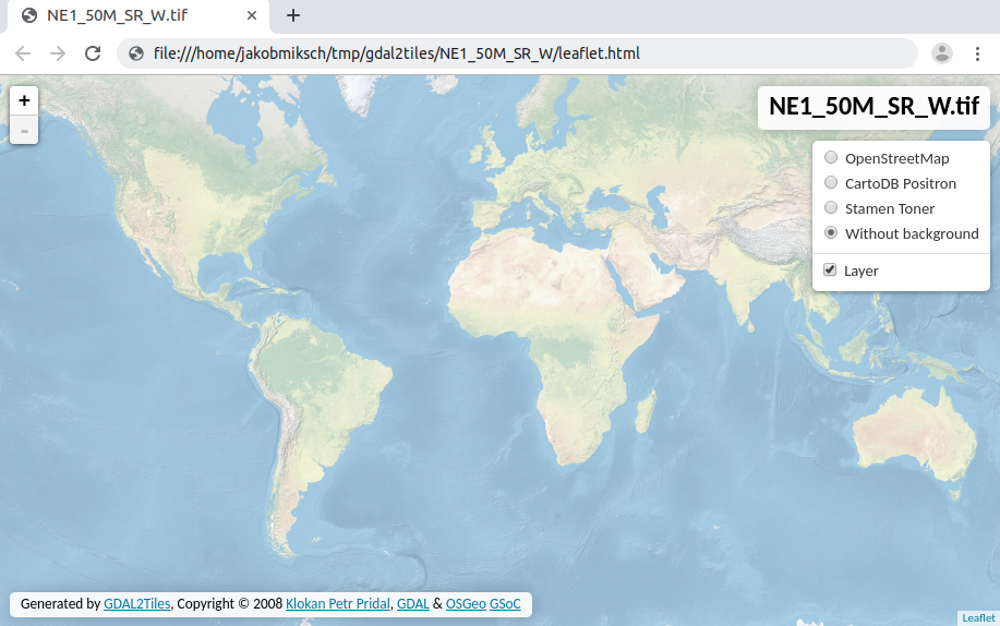
Leaflet based viewer for map tiles
ogrinfo
ogrinfo returns information about a spatial data source. In this example the GeoPackage of NaturalEarth is queried:
ogrinfo \
  natural_earth_vector.gpkg
returns:
INFO: Open of `natural_earth_vector.gpkg'
      using driver `GPKG' successful.
1: ne_10m_admin_0_antarctic_claim_limit_lines (Line String)
2: ne_10m_admin_0_antarctic_claims (Polygon)
3: ne_10m_admin_0_boundary_lines_disputed_areas (Line String)
4: ne_10m_admin_0_boundary_lines_land (Line String)
5: ne_10m_admin_0_boundary_lines_map_units (Line String)
...
This is how you get information about a layer. The option -so stands for “summary only”, This causes that ogr2ogr doesn’t show every single feature:
ogrinfo \
  -so \
  natural_earth_vector.gpkg \
  ne_10m_admin_0_antarctic_claim_limit_lines
This returns important information about the layer like number of features, extent or projection.
INFO: Open of `natural_earth_vector.gpkg'
      using driver `GPKG' successful.

Layer name: ne_10m_admin_0_antarctic_claim_limit_lines
Geometry: Line String
Feature Count: 23
Extent: (-150.000000, -90.000000) - (160.100000, -60.000000)
Layer SRS WKT:
GEOGCS["WGS 84",
    DATUM["WGS_1984",
        SPHEROID["WGS 84",6378137,298.257223563,
            AUTHORITY["EPSG","7030"]],
        AUTHORITY["EPSG","6326"]],
    PRIMEM["Greenwich",0,
        AUTHORITY["EPSG","8901"]],
    UNIT["degree",0.0174532925199433,
        AUTHORITY["EPSG","9122"]],
    AUTHORITY["EPSG","4326"]]
FID Column = fid
Geometry Column = geom
type: String (15.0)
scalerank: Integer (0.0)
featurecla: String (50.0)
The option -al
applies the ogrinfo command to all layers of the data source. This can be useful sometimes, but can also quickly become confusing. In combination with -so the overview of each layer of a datasource will be displayed.
ogrinfo -so -al natural_earth_vector.gpkg
ogr2ogr
The tool ogr2ogr can read, process and convert vector data into other formats. This will be explained in the following mainly using the example of GeoPackage. This is a promising candidate to replace the Shapefile as an exchange format for geodata.
ogr2ogr commands can quickly look very confusing, but are basically built according to the same pattern.
A simple copy:
ogr2ogr \
  -f GPKG output.gpkg \
  input.gpkg
Conversion of the projection to EPSG:3857.
ogr2ogr \
  -t_srs EPSG:3857 \
  -f GPKG output.gpkg \
  input.gpkg
However, the projection of the input data set must be known. Otherwise it can be specified with -s_srs:
ogr2ogr \
  -s_srs EPSG:4326 \
  -t_srs EPSG:3857 \
  -f GPKG output.gpkg \
  input.gpkg
Shapefile
Shapefiles must consists of at least three different files, namely .shp, .dbf and .shx. For OGR is however enough to only reference the .shp file, but the other sidecar files still need to be present. Since GDAL 3.1 it is also possible to read zipped Shapefiles.
If you query a Shapefile with ogrinfo you only get the name of its single layer back. Since that is not very useful, you should explicitly specify the name of the layer in order to obtain the information you want. This is because a Shapefile is both data source and layer at once.
# only return the name of the layer
ogrinfo countries.shp

# returns the information about the layer
ogrinfo countries.shp countries
Quite often many Shapefiles are gathered in a folder. One useful feature of OGR is to recognise this folder as a datasource. In this example all shapefiles are located in the folder my_shapefiles:
my_shapefiles
├── countries.dbf
├── countries.prj
├── countries.shp
├── countries.shx
├── lakes.dbf
├── lakes.prj
├── lakes.shp
└── lakes.shx
The command ogrinfo my_shapefiles yields:
INFO: Open of 'my_shapefiles'
      using driver 'ESRI Shapefile' successful.
1: countries (Polygon)
2: lakes (Polygon)
The single shapefiles are recognised as layers and can therefore be queried indivually by ogrinfo:
# information about a specific layer
ogrinfo my_shapefiles lakes

# summary of all layers in the folder
ogrinfo -al -so my_shapefiles
GPX
GPS or GNSS devices usually provide their data as GPX files. This file can be opened in QGIS, but it always requires some effort. The conversion into a GeoPackage is as follows:
ogr2ogr \
  -f GPKG output.gpkg \
  input.gpx
In the GeoPackage you can find the following layers:
ogrinfo output.gpkg
returns
INFO: Open of `output.gpkg'
      using driver `GPKG' successful.
1: tracks (Multi Line String)
2: track_points (Point)
3: waypoints (Point)
4: routes (Line String)
5: route_points (Point)
If you need this operation more often, you can create a function from it:
function gpx2gpkg {
  input_gpx="$1"
  filename_without_suffix=${input_gpx%.gpx}
  ogr2ogr -f GPKG "$filename_without_suffix".gpkg $input_gpx
}
CSV
Very often you get data in the CSV-format. These can easily be converted into any other format. With the option -oo (“output options”) many settings can be made. In the example below the column names of the coordinates are given. It is important to assign the corresponding coordinate system of the data set using -a_srs.
ogr2ogr \
  -f GPKG output.gpkg \
  input.csv \
  -oo X_POSSIBLE_NAMES=longitude \
  -oo Y_POSSIBLE_NAMES=latitude \
  -a_srs EPSG:4326
The newly created layer is extended by a geometry column. The original columns with the coordinates are retained. If you don’t want this you can prevent it with the option -oo KEEP_GEOM_COLUMNS=NO.
PostGIS
PostGIS is the spatial extension of the PostgreSQL database and is excellent for storing geodata (link to driver).
Export a table:
ogr2ogr \
  -f GPKG output.gpkg \
  PG:dbname="my_database" "my_table"
Export many tables:
ogr2ogr \
  -f GPKG output.gpkg \
  PG:'dbname=my_database tables=table_1,table_3'
Export the whole database to a GeoPackage:
ogr2ogr \
  -f GPKG output.gpkg \
  PG:dbname=my_database
Export the whole database to a folder of Shapefiles:
ogr2ogr \
  -f "ESRI Shapefile" output_folder \
  PG:dbname=my_database
Load data into PostGIS:
ogr2ogr \
  -f "PostgreSQL" PG:dbname="my_database" \
  input.gpkg \
  -nln "name_of_new_table"
During import, the names of the tables and columns are converted to lowercase. However, you can use the -lco LAUNDER=NO option to keep uppercase letters. However, it is recommended to write everything in lower case letters (unless you have good reasons against it).
ogr2ogr \
  -f "PostgreSQL" PG:dbname="my_database" \
  input.gpkg \
  -lco LAUNDER=NO
When reading multi-geometries the following error might occur: ERROR: Geometry type (MultiPolygon) does not match column type (Polygon) This can be solved with the option -nlt PROMOTE_TO_MULTI:
ogr2ogr \
  -f "PostgreSQL" PG:dbname="my_database" \
  input.gpkg \
  -nlt PROMOTE_TO_MULTI
If you have a whole folder full of GeoPackages (or Shapefiles, GeoJSONs, … ). You can load them into PostGIS with a for loop.
for file in *.gpkg;
  do ogr2ogr \
  -f "PostgreSQL" PG:dbname="my_database" \
  $file;
done
Existing tables can be overwritten with the option -lco OVERWRITE=YES:
ogr2ogr \
  -f "PostgreSQL" PG:dbname="my_database" \
  -lco OVERWRITE=YES \
  input.gpkg
This query gives an overview of most parameters that can be used for a Postgres connection:
ogr2ogr \
-f GPKG output.gpkg \
PG:"
  dbname=my_database
  host=localhost
  port=5432
  user=user_name
  password=my_password
  schemas=schema1
  tables=table1,table2"
It is even possible to write a Postgres Dump without even having PostgreSQL database.
Query and Filter Data
ogr2ogr can also filter and edit geodata. A common application is the limitation of a data set to a certain area. This can be created with the option -spat:
ogr2ogr \
  -spat -13.931 34.886 46.23 74.12 \
  -f GPKG output.gpkg \
  natural_earth_vector.gpkg
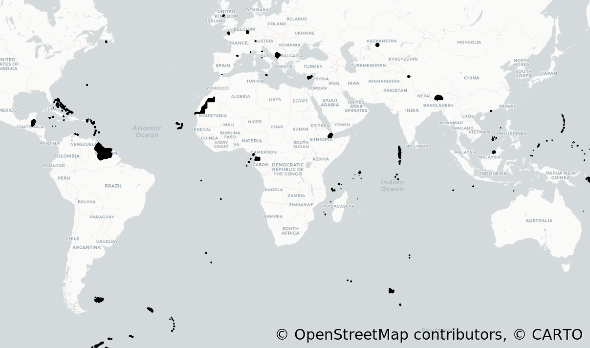
If you only want certain features of a layer, you can define them with -where. This example only returns countries with less than 1 million inhabitants:
ogr2ogr \
  -where "\"POP_EST\" < 1000000" \
  -f GPKG output.gpkg \
  natural_earth_vector.gpkg \
  ne_10m_admin_0_countries
The conditions following the -where must be in ". If there are more " in it, however, these must be escaped with a \. This is the result on the map:
The two options -spat and -where can of course be combined. This then returns the countries in Europe under 1 million inhabitants:
ogr2ogr \
  -where "\"POP_EST\" < 1000000" \
  -spat -13.931 34.886 46.23 74.12 \
  -f GPKG output.gpkg \
  natural_earth_vector.gpkg \
  ne_10m_admin_0_countries
With the option -sql you can make queries using SQL. Although SQL is actually intended for databases, you can use ogr2ogr to apply it to any type of dataset.
The following example uses this CSV file as input:
ID,Name,latitude,longitude
1,Salzburg, 47.8, 13.0
2,Heidelberg, 49.4, 8.7
3,Trondheim, 63.4, 10.4
With this command only cities with a latitude of less than 50° are displayed:
ogr2ogr \
-f GPKG output.gpkg \
cities.csv \
-sql "SELECT * FROM cities WHERE latitude < 50" \
-oo X_POSSIBLE_NAMES=longitude \
-oo Y_POSSIBLE_NAMES=latitude \
-a_srs EPSG:4326
Very often SQL query can become quite long. ogr2ogr offers the useful functionality that the SQL query can be written into a separate text file which can be referenced within the ogr2ogr command. The latter example can hence be separated. This would be the textfile with the SQL query:
SELECT *
  FROM cities
 WHERE latitude < 50
And this would be the ogr2ogr command where the textfile is referenced within the -sql option using a @ sign:
ogr2ogr \
-f GPKG output.gpkg \
cities.csv \
-sql @path/to/query.sql \
-oo X_POSSIBLE_NAMES=longitude \
-oo Y_POSSIBLE_NAMES=latitude \
-a_srs EPSG:4326
There is not the “one” SQL, but there are different dialects. ogr2ogr can always take the dialect of the corresponding input data source. For example Postgres-SQL if it is a Postgres/PostGIS database. Alternatively also its own OGR SQL or SQLite SQL. This can be set with the option -dialect.
With SQL you can create geometries from coordinates. In the following example, a non-spatial SQLite table is converted into a spatial GeoPackage. The function MakePoint() creates a valid geometry from the coordinates.
ogr2ogr \
  -f GPKG output.gpkg \
  input.sqlite \
  -sql \
  "SELECT
     *,
     MakePoint(longitude, latitude, 4326) AS geometry
   FROM
     my_table" \
  -nln "location" \
  -s_srs EPSG:4326
ogr2ogr: More Functions
With -append you can merge different layers. However, these layers must have the same structure. The following example takes all GeoPackages in one folder and merges them:
for geopackage in *gpkg; do
  ogr2ogr \
  -f "GPKG" combined.gpkg \
  -append \
  $geopackage
done
With the option -progress you can see how much percent of the conversion has already been done. This makes sense especially for operations that take a long time.
The –debug ON option displays a lot of additional information when the command is executed. This is especially useful if the command does not work and you want to find the error.
GDAL/OGR can also process files which are located in the internet. For example, this command converts a remote GeoJSON into a local GeoPackage:
ogr2ogr \
-f GPKG chapters.gpkg \
https://raw.githubusercontent.com/maptime/maptime.github.io/master/_data/chapters.json
Virtual Vector Format
Similar to raster there is a driver for vectors with which you can create virtual vector files (see VRT). Basically, one or more vector data sources are referenced by an XML file. But the VRT file is not only a simple link to the referenced file, numerous conversions can be performed. For example, fields can be renamed or omitted or the coordinate system can be re-projected.
The following VRT creates a simple reference to a GeoJSON available on the Internet:
<OGRVRTDataSource>
  <OGRVRTLayer name="my_new_layer_name">
    <SrcDataSource relativeToVRT="0" shared="1">https://raw.githubusercontent.com/maptime/maptime.github.io/master/_data/chapters.json</SrcDataSource>
    <SrcLayer>chapters</SrcLayer>
  </OGRVRTLayer>
</OGRVRTDataSource>
This VRT can be processed normally with ogrinfo or ogr2ogr or can be opened with QGIS. These XML files are usually created by hand. However, there is also a command line tool called ogr2vrt.py which creates a basic XML structure which can be edited manually. This tool is not part of the normal GDAL installation, it has to be downloaded from the repository. The application works as follows:
ogr2vrt.py \
  https://raw.githubusercontent.com/maptime/maptime.github.io/master/_data/chapters.json \
  chapters.vrt
creates this VRT-file:
<OGRVRTDataSource>
<OGRVRTLayer name="chapters">
<SrcDataSource relativeToVRT="0" shared="1">https://raw.githubusercontent.com/maptime/maptime.github.io/master/_data/chapters.json</SrcDataSource>
<SrcLayer>chapters</SrcLayer>
<GeometryType>wkbPoint</GeometryType>
<LayerSRS>GEOGCS["WGS 84",DATUM["WGS_1984",SPHEROID["WGS 84",6378137,298.257223563,AUTHORITY["EPSG","7030"]],AUTHORITY["EPSG","6326"]],PRIMEM["Greenwich",0,AUTHORITY["EPSG","8901"]],UNIT["degree",0.0174532925199433,AUTHORITY["EPSG","9122"]],AXIS["Latitude",NORTH],AXIS["Longitude",EAST],AUTHORITY["EPSG","4326"]]</LayerSRS>
<Field name="location" type="String" src="location"/>
<Field name="title" type="String" src="title"/>
<Field name="twitter" type="String" src="twitter"/>
<Field name="website" type="String" src="website"/>
<Field name="meetup" type="String" src="meetup"/>
<Field name="comingSoon" type="String" src="comingSoon"/>
<Field name="organizers" type="String" src="organizers"/>
<Field name="moreInfo" type="String" src="moreInfo"/>
<Field name="github" type="String" src="github"/>
<Field name="facebook" type="String" src="facebook"/>
</OGRVRTLayer>
</OGRVRTDataSource>
This file actually only copies the properties that the layer already has and is primarily suitable as a template for your own changes. For example you can assign a new name to a column without changing the original data source: <Field name="My new Name" type="String" src="title"/>
VRTs have a variety of useful applications. For example, you can convert connections to databases or webservices to a VRT. Hence they are wrapped into a single file. Coordinate columns in Excel files can also be referenced, allowing them to be processed as spatial data or displayed (e.g. QGIS).
Python
There is a gdal package for Python. However, the syntax of the functions is very close to the C++ API and therefore rather difficult. For raster data there is the wrapper rasterio. For vector data there is the wrapper fiona. The documentation describes for which cases fiona is suitable.
You can also access ogr2ogr from the command line inside Python. To simplify this, you can use the script ogr2ogr.py (link). This is called as follows:
import ogr2ogr

ogr2ogr.main([
  'ogr2ogr',
  '-f', 'GPKG', 'output.gpkg' ,
  'input.gpkg'
])
Docker
Besides the regular installation, we can use the GDAL/OGR utilities via Docker. This has the advantage that we can use the latest version, or use any older version. There are five docker images available:
alpine-normalalpine-smallalpine-ultrasmallubuntu-fullubuntu-small
Their detailed description are in the offical README. They contain different numbers of drivers and have a different download size. Hence, we need to think first which formats we would like to open and then decide which image we choose.
The following examples use alpine-small, because we only need the GeoPackage and the Postgres driver. Make sure you install docker on your computer. Navigate to a directory that contains your geodata. In our case we have one GeoPackage file called sample.gpkg.
The following command opens a sh shell inside the docker container. We are mounting the current host directory to the /data directory inside the docker container.
docker run \
  -t \
  -i \
  -v $(pwd):/data \
  osgeo/gdal:alpine-small-latest \
  sh
All GDAL/OGR command are available in this shell. Hence, we can get information of the file or do a conversion:
# get version of GDAL/OGR
ogrinfo --version

# get basic information of GeoPackage
ogrinfo /data/sample.gpkg

# convert 'layer_1' of our GeoPackage into GeoJSON
ogr2ogr \
  -f GeoJSON \
  /data/out.json \
  /data/sample.gpkg \
  layer_1
The last command creates a new file that will appear in our host directory from where we started the shell. We can also perform commands directly without opening up the docker shell. The following command converts a layer of our GeoPackage to a Shapefile.
docker run \
  -v $(pwd):/data osgeo/gdal:alpine-small-latest \
  ogr2ogr \
    -f "ESRI Shapefile" \
    /data/out.shp \
    /data/sample.gpkg \
    layer_1
Accessing a local database requires the setting --network=host for our docker command. However, this seems to work only for Linux machines. This thread discusses alternatives for Windows and Mac.
docker run \
  --network=host \
  -t \
  -i \
  -v $(pwd):/data \
  osgeo/gdal:alpine-small-latest \
  ogr2ogr \
    -f GeoJSON \
    /data/db_export.geojson \
    PG:"
    dbname=my_database
    host=localhost
    port=5432
    user=postgres
    password=postgres" \
    my_table
Bonus - Features
GDAL/OGR has some rather unknown function, which however are probably not needed that often.
Viewshed: From GDAL 3.1 on there is a function that can compute the visible area on a digital elevation model (DEM) from the location of an observer.
GeoCoding: The SQLite dialect offers a function for geocoding. Hence, a name of a place can be give as input and the coordiante of the location will be returned. For example, we can take this CSV file as input:
id,name,country
1,Salzburg,Austria
2,Heidelberg,Germany
3,Trondheim,Norway
From this list, we request the location for each city and save it into a GeoPackage.
ogr2ogr \
  -f GPKG output.gpkg \
  geocode.csv \
  -dialect sqlite \
  -sql "
  SELECT
    id,
    name,
    country,
    ogr_geocode(name || ', ' || country) AS geometry
  FROM geocode"
The SQLite dialect also offers the function ogr_geocode_reverse() which takes a name as input and returns its coordinates.
Thanks to the Developers
As already mentioned GDAL/OGR is free and OpenSource. At this point I would like to thank Frank Warmerdam who started the project and Even Rouault who meanwhile became the main developer. And of course the many other contriubutors who are developing the project further and keep it running.
If you find GDAL/OGR useful please consider supporting the work of the project’s maintainer Even Rouault (Spatialys).
You can also buy a GDAL T-Shirt. The profit of the sale is donated to OSGeo. That is the umbrella organisation that supports GDAL and many other geospatial open source projects.
Links
- Website of GDAL/OGR
- Sourcecode of GDAL/OGR
- Talk - Introduction to OGR with Python by Nikolai Janakiev
- Talk - Introduction to GDAL with Python by Hannah Augustin
- Talk - State of GDAL 2019 by Even Rouault
- Talk - An Introduction to GDAL bx Robert Simmon
- extensive Introduction to GDAL
- Talk - GDAL Tips and Tricks
- blog posts by Koko Alberti
- blog posts by Hannes Kröger
- book GeoSpatial Power Tools (2012) by Tyler Mitchell
- video tutorials by “Making Sense Remotely”
- Twitter account @gdaltips with many useful GDAL/OGR commands
- Tutorial about Cloud Optimized GeoTIFF (COG) as Jupyter Notebook by OpenTopography
- Presentation about GDAL/OGR commandline tools by Jakob Miksch
CheatSheets
- by Garret - glw
- by BostonGIS
- by Nathan Shaw
- by Derek Watkins - dwtkns
- by Lyzi Diamond
Revisions of this Post
- 2021-04-11: Add docker instructions
- 2020-05-10: Add virtual vector format (VRT)
- 2019-12-16: Additions to Shapefile, SQL, GeoCoding, Viewshed,
ogr2ogroptions, GeoJSON Download - 2019-09-20: First version of this post
This post was originally written in German. It was translated with www.DeepL.com/Translator and manually revised by the author.